PyTorch and Submitit

Defining models, datasets and functions

If you’re doing something relatively simple, Dask has integrations with Scikit-Learn and XGBoost. You can also pass PyTorch models into Scikit-Learn with Skorch and TensorFlow models with SciKeras.

But if you need to do something more complex, using SubmitIt to remotely execute code gives us the low level control to implement whatever bespoke algorithm we want and have it accelerated by remote GPUs.

In this example we’re going to write our own PyTorch functions to train a custom model on the CIFAR dataset. While we could do this with Skorch, we hope that this example gives you some idea of how Dask can be flexible enough for any applications that you need.

Content adapted from the PyTorch CIFAR10 Tutorial

import torch
import torchvision
import torchvision.transforms as transforms
import torch.multiprocessing as mp

# Define data transformations
transform = transforms.Compose([
    transforms.ToTensor(),
    transforms.Normalize((0.5, 0.5, 0.5), (0.5, 0.5, 0.5))
    ])

# Define dataset and dataloader
batch_size = 1024
trainset = torchvision.datasets.CIFAR10(root='./data', train=True,
                                        download=True, transform=transform)
validset = torchvision.datasets.CIFAR10(root='./data', train=False,
                                        download=True, transform=transform)

# Note that we need to set the multiprocessing context so that PyTorch doesn't get
# PyTorch likes to use 'forking' while Dask uses 'spawn'
trainloader = torch.utils.data.DataLoader(trainset, batch_size=batch_size,
                                          shuffle=True, num_workers=16, multiprocessing_context=mp.get_context("fork"))
validloader = torch.utils.data.DataLoader(validset, batch_size=batch_size,
                                          shuffle=True, num_workers=16, multiprocessing_context=mp.get_context("fork"))

Files already downloaded and verified
Files already downloaded and verified

/apps/mambaforge/envs/dsks_2024.06/lib/python3.10/site-packages/torch/utils/data/dataloader.py:558: UserWarning: This DataLoader will create 16 worker processes in total. Our suggested max number of worker in current system is 8, which is smaller than what this DataLoader is going to create. Please be aware that excessive worker creation might get DataLoader running slow or even freeze, lower the worker number to avoid potential slowness/freeze if necessary.
  warnings.warn(_create_warning_msg(

Note that this cell may warn us that there is a mismatch between our requested resources and the number of worker processes. This is ok, as we have sized this DataLoader to match the Dask worker that we request later on.

import torch.nn as nn
import torch.nn.functional as F

# Define loss function
criterion = nn.CrossEntropyLoss()

# Define a simple conv net
class Net(nn.Module):
    def __init__(self):
        super().__init__()
        # Convolutional layers
        self.conv1 = nn.Conv2d(3, 16, 3, stride=2, padding=1)
        self.conv2 = nn.Conv2d(16, 16, 3, stride=1, padding=1)
        self.conv3 = nn.Conv2d(16, 32, 3, stride=2, padding=1)
        self.conv4 = nn.Conv2d(32, 32, 3, stride=1, padding=1)
        self.conv5 = nn.Conv2d(32, 64, 3, stride=2, padding=1)
        self.conv6 = nn.Conv2d(64, 64, 3, stride=1, padding=1)
        
        # Fully connected layers
        self.fc1 = nn.Linear(4 * 4 * 64, 4 * 64)
        self.fc2 = nn.Linear(4 * 64, 64)
        self.fc3 = nn.Linear(64, 10)

    def forward(self, x):
        # Pass through convolution layers
        x = F.relu(self.conv1(x))
        x = F.relu(self.conv2(x))
        x = F.relu(self.conv3(x))
        x = F.relu(self.conv4(x))
        x = F.relu(self.conv5(x))
        x = F.relu(self.conv6(x))

        # Flatten all dimensions except batch
        x = torch.flatten(x, 1)  

        # Pass through fully connected layers
        x = F.relu(self.fc1(x))
        x = F.relu(self.fc2(x))
        x = self.fc3(x)
        return x

This train function will load any saved state for the provided model, then train for a number of epochs. When its done it will then save the state and return the average loss of the last epoch.

import torch.optim as optim
from tqdm.notebook import tqdm


# loader: train dataloader
# arch: model archetechture for training
# path: model path for load and save
# load: whether to load model from path
# save: whether to save model to path
# test: only run one batch for testing
# error: throw an assertion error
# return: average loss of epoch or loss of one batch if testing
def train(loader, arch=Net, path="./model", epochs=1, load=False, save=True, test=False):
    model = arch()
    optimizer = optim.Adam(model.parameters(), lr=3e-4)
    device = "cuda" if torch.cuda.is_available() and not test else "cpu"
    
    # Load state from disk so that we can split up the job
    if load: 
        state = torch.load(path, map_location="cpu")
        model.load_state_dict(state["model"])
        model.to(device)
        optimizer.load_state_dict(state["optimizer"])
    else:
        model.to(device)
    
    # A typical PyTorch training loop
    model.train()
    for _ in range(epochs):
        running_loss = 0
        
        for i, (inputs, labels) in enumerate(loader):
            # put the inputs on the device
            inputs, labels = inputs.to(device), labels.to(device)

            # zero the parameter gradients
            optimizer.zero_grad()

            # forward + backward + optimize
            outputs = model(inputs)
            loss = criterion(outputs, labels)
            loss.backward()
            optimizer.step()
            running_loss += loss.detach().item()
    
    # Save model after each epoch
    if save:
        torch.save({
            "model": model.state_dict(),
            "optimizer": optimizer.state_dict()
            }, path)
    
    return running_loss / len(loader) if not test else loss.detach().item()

This valid function will load the state of the model we’ve defined, then calculate the average loss and accuracy over the dataset.

# loader: train dataloader
# arch: model archetechture for validating
# path: model path for load and save
# return: average loss and accuracy of epoch
def valid(loader, arch=Net, path="./model"):
    # Initialise device
    model = arch()
    device = "cuda" if torch.cuda.is_available() else "cpu"

    # Load state from disk so that we can split up the job
    state = torch.load(path, map_location="cpu")
    model.load_state_dict(state["model"])
    model.to(device)
    model.eval()
    
    # A typical PyTorch validation loop
    running_loss = 0
    correct = 0
    total = 0
    with torch.no_grad():
        for i, (inputs, labels) in enumerate(loader):
            # put the inputs on the device
            inputs, labels = inputs.to(device), labels.to(device)

            # forward
            outputs = model(inputs)
            
            # loss
            loss = criterion(outputs, labels)
            running_loss += loss.detach().item()
            
            # accuracy
            _, predicted = torch.max(outputs.data, 1)
            total += labels.size(0)
            correct += (predicted == labels).sum().item()

    return running_loss / len(loader), correct / total

Testing locally

train(trainloader, test=True)

2.065371513366699

Training with a `SubmitIt`

import submitit

# Define where we'd like submitit to place our logs
executor = submitit.AutoExecutor(folder='~/submitit_logs')

# Define the parameters of our slurm job
# Just like Dasks' job_extra_directives, additional_parameters allows us to specify things that submitit doesn't support directly
executor.update_parameters(timeout_min=30, mem_gb=128, cpus_per_task=16, slurm_partition="BigCats", slurm_additional_parameters={"gres": "gpu:2g.10gb:1"})

# First test offloading before we run the full training loop
executor.submit(train, trainloader, test=True).result()

2.058852434158325

Finally we can bring everything together and run our training loop.

# Run the training loop
epochs = 5
with tqdm(total=(epochs)) as pbar:
    for epoch in range(epochs):
        train_loss = executor.submit(train, trainloader, load=(epoch > 0)).result()
        valid_loss, accuracy = executor.submit(valid, validloader).result()
        pbar.update()
        pbar.set_postfix(loss=train_loss)
        print( f"epoch: {epoch}, train_loss: {train_loss : .3f}, valid_loss: {valid_loss : .3f}, accuracy: {accuracy : .3f}")

epoch: 0, train_loss:  2.273, valid_loss:  2.119, accuracy:  0.224
epoch: 1, train_loss:  1.998, valid_loss:  1.928, accuracy:  0.294
epoch: 2, train_loss:  1.872, valid_loss:  1.807, accuracy:  0.333
epoch: 3, train_loss:  1.770, valid_loss:  1.720, accuracy:  0.365
epoch: 4, train_loss:  1.702, valid_loss:  1.654, accuracy:  0.385

Note how in this example we offload every epoch as its own function. If your model or dataset is large, you may find it more efficient to submit multiple epochs to be trained per batch. In doing so, consider specifying larger GPU sizes and using the lion qos if the 30 minute joblength for Cheetah is too short.

Measuring the offloading overhead

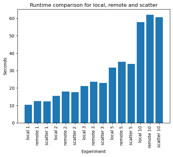
Offloading tasks doesn’t come for free, there is an initial cost associated with sending the data to a remote device. Let’s compare the time it would take to train a Resnet18 on CIFAR for a range of epochs comparing a local GPU, a remote GPU using Dask and a remote GPU using Dask with a scattered dataset. For this expriment we will not bother saving the weights afterwards since this should be relatively constant between methods.

Note that this test was run directly on the compute node to gain direct access to the GPUs to measure overheads. You will only be able to mimic our results for the final graph if you’re running with an inbuilt GPU (Tabby service) since it compares reserved GPUs with Dask driven GPU jobs. Running this cell in a lion service will likely freeze the notebook since you’d have no accelleration.

from torchvision.models import resnet18
from time import time

# Store times in arrays
local = []
remote = []
scatter = []

# Test some number of epochs
epoch_list = [1, 2, 3, 5, 10]
with tqdm(total=(len(epoch_list) * 3)) as pbar:
    for num_epochs in epoch_list:
        
        # Local GPU
        start = time()
        train(trainloader, arch=resnet18, epochs=(num_epochs + 1), save=False)
        local.append(time() - start)
        pbar.update()
        
        # Remote GPU
        start = time()
        client.submit(train, trainloader, arch=resnet18, epochs=(num_epochs + 1), save=False).result()
        remote.append(time() - start)
        pbar.update()
        
        # Remote GPU with scatter
        start = time()
        trainloader_future = client.scatter(trainloader)
        client.submit(train, trainloader_future, arch=resnet18, epochs=(num_epochs + 1), save=False).result()
        scatter.append(time() - start)
        pbar.update()

import matplotlib.pyplot as plt
from itertools import chain

data = list(chain(*zip(local, remote, scatter)))
columns = []
for num_epochs in epoch_list:
    for test in ["local", "remote", "scatter"]:
        columns.append(test + " " + str(num_epochs))

plt.bar(range(len(data)), data, tick_label=columns)
plt.xticks(rotation=90)
plt.xlabel("Experiment")
plt.ylabel("Seconds")
plt.title("Runtime comparison for local, remote and scatter")
plt.show()

From this experiment we can see that the cost associated with running code remotely is small, and the impact decreases with the size of the function that we submit. It also shows that it always makes sense to scatter large objects before computing, even for small jobs.

client.shutdown()

Defining models, datasets and functions

Testing locally

Training with a SubmitIt

Measuring the offloading overhead

Training with a `SubmitIt`